Magnetic Modeling

As magnetic components such as inductors or transformers are key components in power converters, SIMBA allows the user to model these components in a special magnetic circuit domain. In the magnetic library, the user can find the elements to model the magnetic components:

• windings which form the interface between the electrical and the magnetic domain,
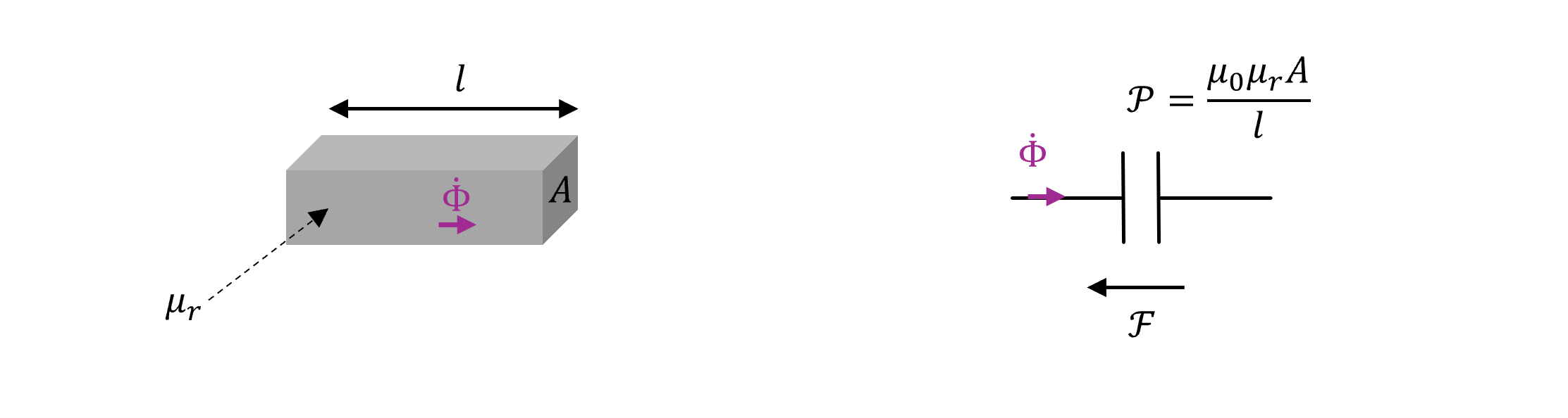
• cores and air gaps which are based on an permeance element, for the magnetic circuit.

Modeling approach

SIMBA uses a gyrator-capacitor method, first introduced by R.W. Buntenbach ¹ and fully described by Hamill ², which is more convenient to model complex magnetive components such as coupled inductors or transformers with multiple windings. In this approach, magnetic paths are modeled by capacitive circuits and windings are represented by gyrator two-ports.

This approach is commonly used through the Bond-Graph approach ³. The magnetic motive force (mmf) written $\mathcal{F}$ is retained as the effort variable and the flux rate ($d\Phi/dt$) written $\dot\Phi$ is retained as the flow variable. The conversion from the electrical to the magnetic domain (and vice versa) such as with a N-turn winding is modeled with a N-ratio gyrator.

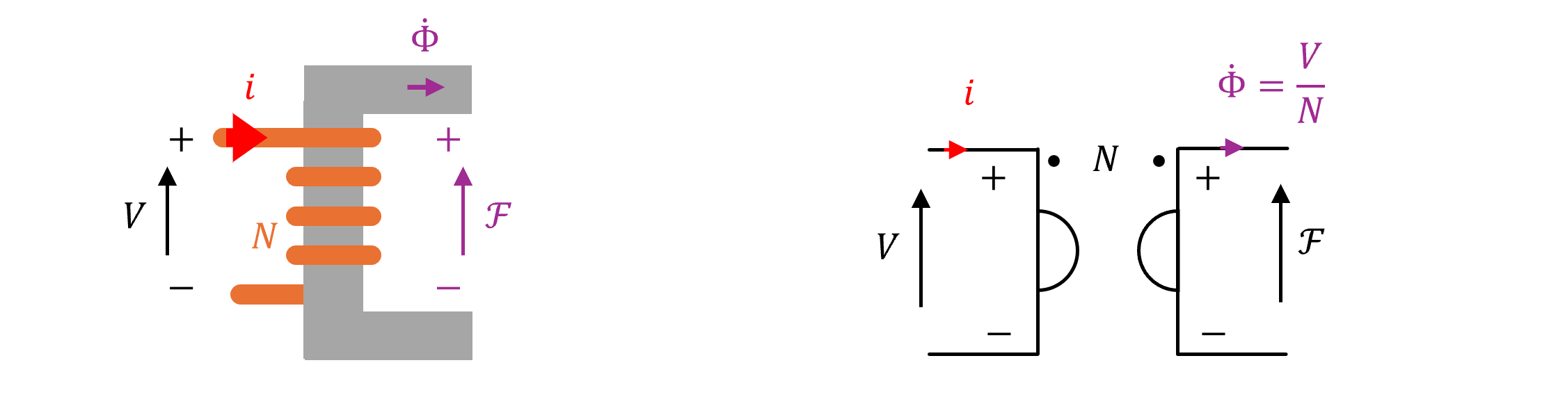
A gyrator can be compared to a N-ratio transformer. But, unlike the transformer where the effort variable of the primary side is linked to the effort variable of the secondary side ($V_s = N \times V_p$), the effort variable of the secondary side is linked to the flow variable of the primary side (and vice versa) with the following relations:

$$V = N \times \dot \Phi$$

$$\mathcal{F} = N \times i$$

The product of effort and flow variables is the power so this approach keeps the power from one domain to the other.

	Magnetic			Electrical
mmf	$\mathcal{F}$	(A)	Voltage	$v$	(V)
Flux rate	$\dot \Phi$	(Wb/s)	Current	$i$	(A)
Permeance	$\mathcal{P}$	(H)	Capacitance	$C$	(F)
Flux	$\Phi = \int{\dot \Phi ~dt}$	(Wb)	Charge	$q = \int{i~dt} ~ (C)$	(C)
Permeability	$\mu = \mu_0 \mu_r$	(H/m)	Permittivity	$\epsilon = \epsilon_0 \epsilon_0$	(F/m)
Power	$P = \mathcal{F} \times \dot \Phi$	(W)	Power	$P = v \times i$	(W)
Energy	$E = \int{Fd\Phi}$	(J)	Energy	$E = \int{v dq}$	(J)

With the electrical - magnetic analogy shown in the table above, magnetic flux is analogous to electric charge, not electric current. In the electrical domain, voltage $v$ pushes charge around the electrical circuit causing a flow of current ($i = dq/dt$), in the magnetic domain the mmf $F$ pushes flux around the magnetic circuit, causing a flow of flux rate ($d\Phi/dt$). Thus, magnetic permeance becomes analogous to electrical capacitance.

This may also be seen with the following equations:

$$\Phi = \mathcal{F} / \mathcal{R} = \mathcal{P} \times \mathcal{F}$$

where $\mathcal{P} = 1/\mathcal{R}$ is the permeance.

Finally, it comes:

$$\dot \Phi = \mathcal{P} \frac{d\mathcal{F}}{dt}$$

The figure below shows the model of a magnetic flux path using a permeance:

Convention

The winding gyrator element in SIMBA uses the following convention shown in figure below. Considering the flux convention defined by the arrow, When the flux rate is positive it leads to a positive voltage as shown in the figure (in other words the positive potential is on the flux arrowhead side):

Example of a transformer modeling

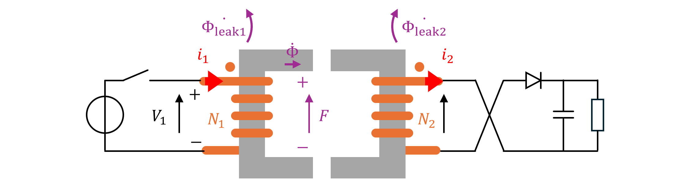
The modeling of a 2-windings (for a Flyback application for example) is proposed below, following three different steps:

1. consideration of the magnetic circuit (reluctance / permeance),
2. consideration of the magnetic flux leakages,
3. consideration of the magnetic losses.

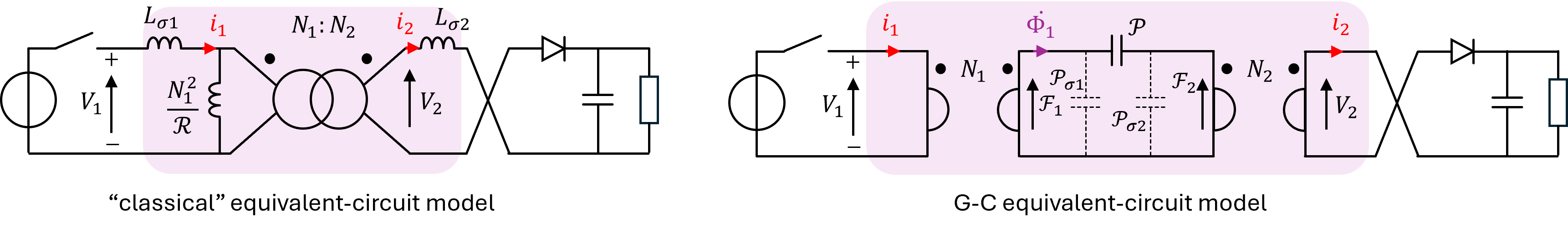
Step 1: Consideration of the magnetic circuit

In this first step, leakages are neglected as well as the magnetic losses. The figure below shows:

• on the left the "classical" equivalent-circuit model of the transformer with the magnetizing inductor $N^2/\mathcal{R}$,
• on the right the gyrator - capacitor (G-C) equivalent-circuit model with the permeance capacitor $\mathcal{P}$.

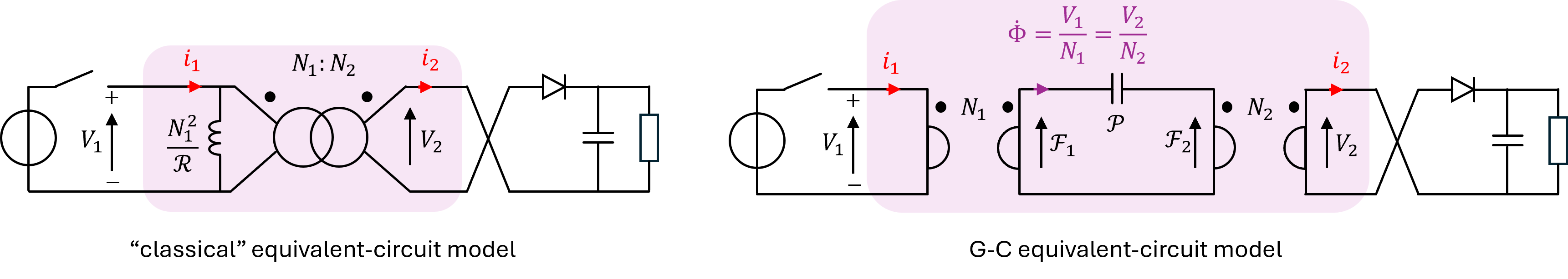
With the considered conventions, the following equations can be written:

$$\dot \Phi = \frac{V_1}{N_1} = \frac{V_2}{N_2}$$

$$\dot \Phi = \mathcal{P} \frac{d}{dt}(\mathcal{F}_1 - \mathcal{F}_2)$$

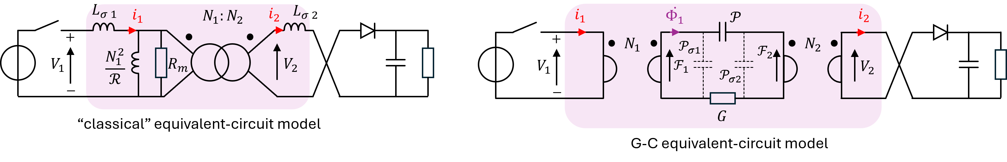
Step 2: Consideration of the magnetic flux leakages

In this second step, the magnetic losses are still neglected. The figure below shows the "classical" equivalent-circuit model (on the left) and the G-C equivalent circuit model (on the right). This last one includes permeances $P_1$ and $P_2$ to represent the leakage paths associated with windings $N_1$ and $N_2$.

Note

It can be noted the dual representation of the leakage flux paths:

• in the "classical" equivalent-circuit model, they are represented by inductors $L_{\sigma1}$, $L_{\sigma2}$ and connected in series with each winding and lead to drop voltages,
• in the G-C equivalent circuit model, they are represented by permeance capacitors $\mathcal{P}_{\sigma1}$, $\mathcal{P}_{\sigma2}$ connected in parallel to the mmf $\mathcal{F}_1$ and $\mathcal{F}_2$ and lead to leakage flux rates.

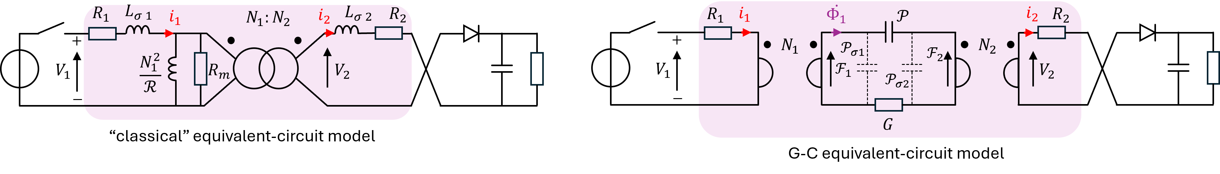
Step 3: Consideration of the magnetic losses

In this third step, the magnetic losses are considered and modeled by $R_m$ in parallel of the magnetizing inductor in the "classical" equivalent-circuit model and a by $G$ in series with the permeance $\mathcal{P}$ in the G-C equivalent circuit model.

In both cases, the winding resistances $R_1$ and $R_2$ are modeled in the electrical domain as shown in figure below.

References

---

1. R.W. Buntenbach, Improved circuit models for inductors wound on dissipative magnetic cores, in Proc. 2nd Asilomar Conference on Circuits & Systems, Pacific Grove, CA, Oct. 1968 (IEEE publ. no. 68C64-ASIL), pp. 229-236. ↩

2. D. C. Hamill, Lumped equivalent circuits of magnetic components: the gyrator-capacitor approach, in IEEE Transactions on Power Electronics, vol. 8, no. 2, pp. 97-103, April 1993. ↩

3. D. Kamopp and R. Rosenberg, System Dynamics A Unlfred Approach New York: Wiley, 1975. ↩