Interface Overview

Installation, Requirements and Activation

Simply run SIMBA.exe on any modern Windows PC. A one-time activation process that requires an internet connection is required.

Interface Overview

At its heart, SIMBA is a circuit simulator. Like many other circuit simulators, SIMBA adopts a common user interface and layout of a Design and Library explorer on the left, showing all of the designs and models you have access to, a circuit editor in the center and a property panel on the right.

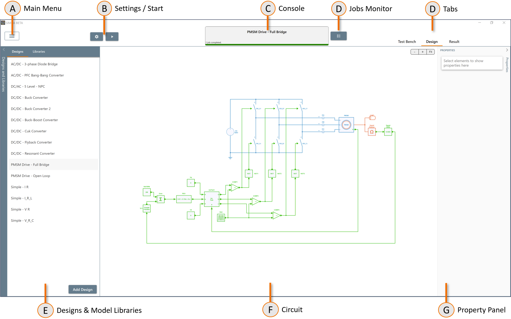
The interface of SIMBA is divided into different views:

• Functionnalities pannel
• Circuit view
• Property pannel

Design Tab

The design tab is the center of your modeling experience.

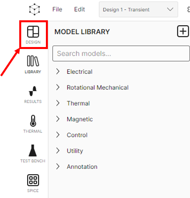
Design Explorer

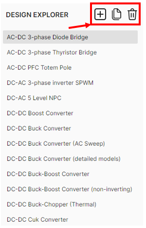
In SIMBA, a single project file can contain multiple designs, results, test benches and scripts.

In the Design Explorer, when you move the pointer over the explorer, you can see and use Add Design, Duplicate Design or C buttons to create, duplicate or remove any design.

Select one of the design in the list to open it in the Circuit editor.

Circuit Editor

Add and Move Models

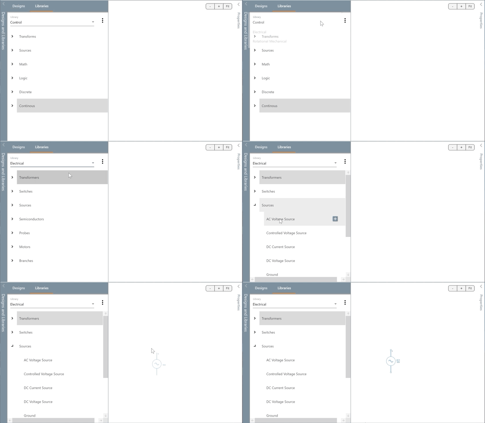
Simba Model Libraries contains dozens of electrical, mechanical, and control models.

To open the library list, select the corresponding tab on the left.

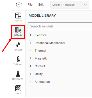
To add a model to a circuit, simply double-click on it in the Library explorer or drag and drop it.

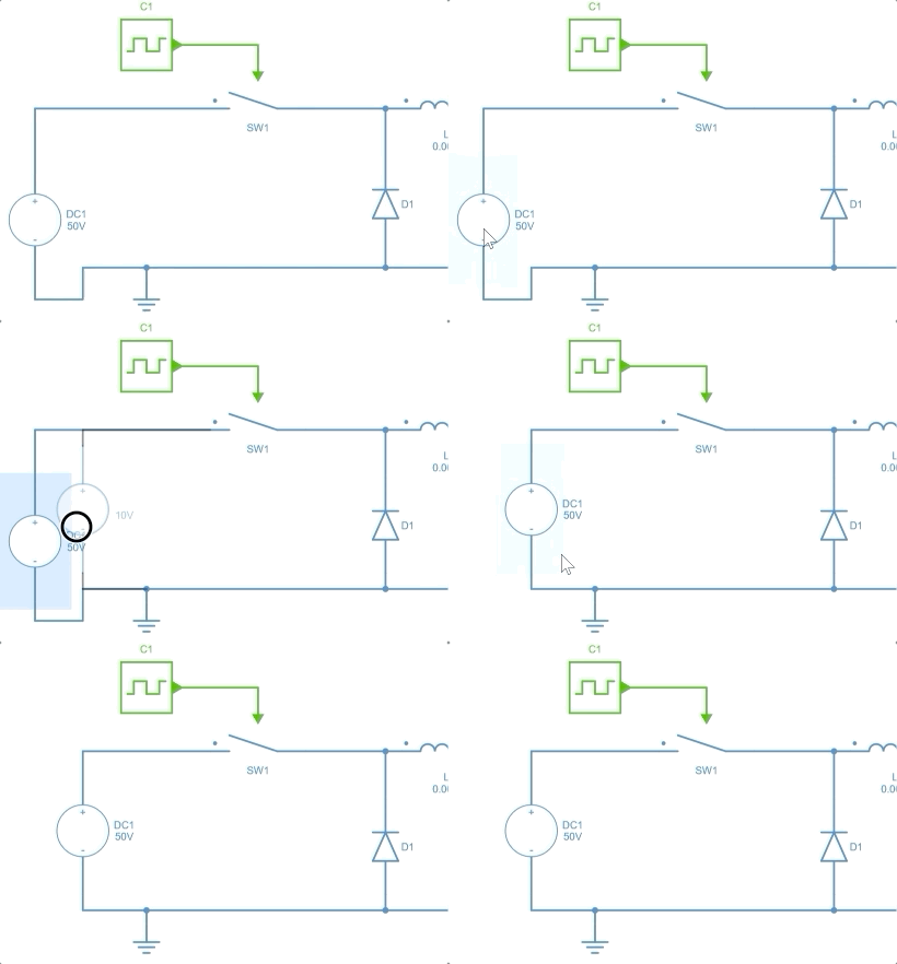
To move a model, simply drag and drop it. Moving devices keep connections.

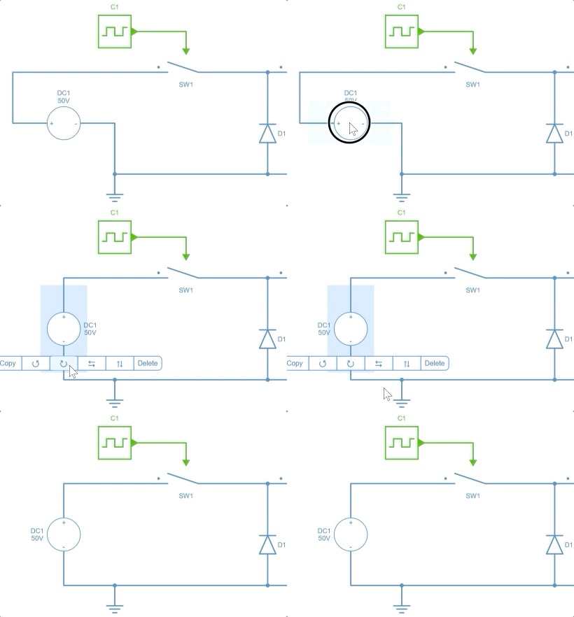
Rotation and flip options are available when a device is selected.

Connect Models

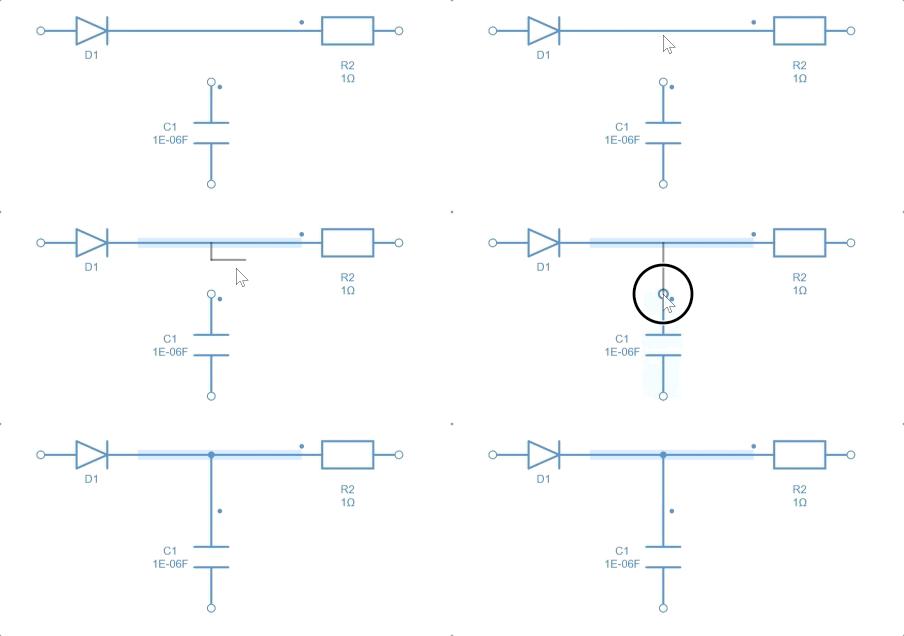
To connect models, click on a pin and drag the mouse while holding the left mouse button to the destination.

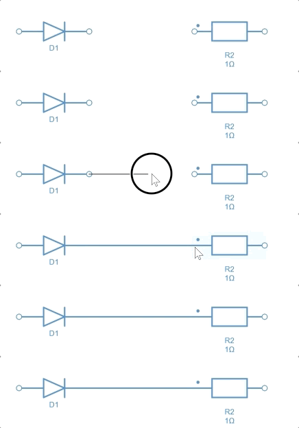
It is also possible to use the + button available when a connector is selected.

Disable / Enable

It is possible to enable and disable devices by clicking the corresponding button in the context menu. Disabled devices are greyed out and are excluded from the simulation.

Label

Labels can be used to connect different parts of a circuit without using connectors. To add a label, simply select a connector and click on the Label button.

Labels are also available in the Utility library.

Scopes and Parameters

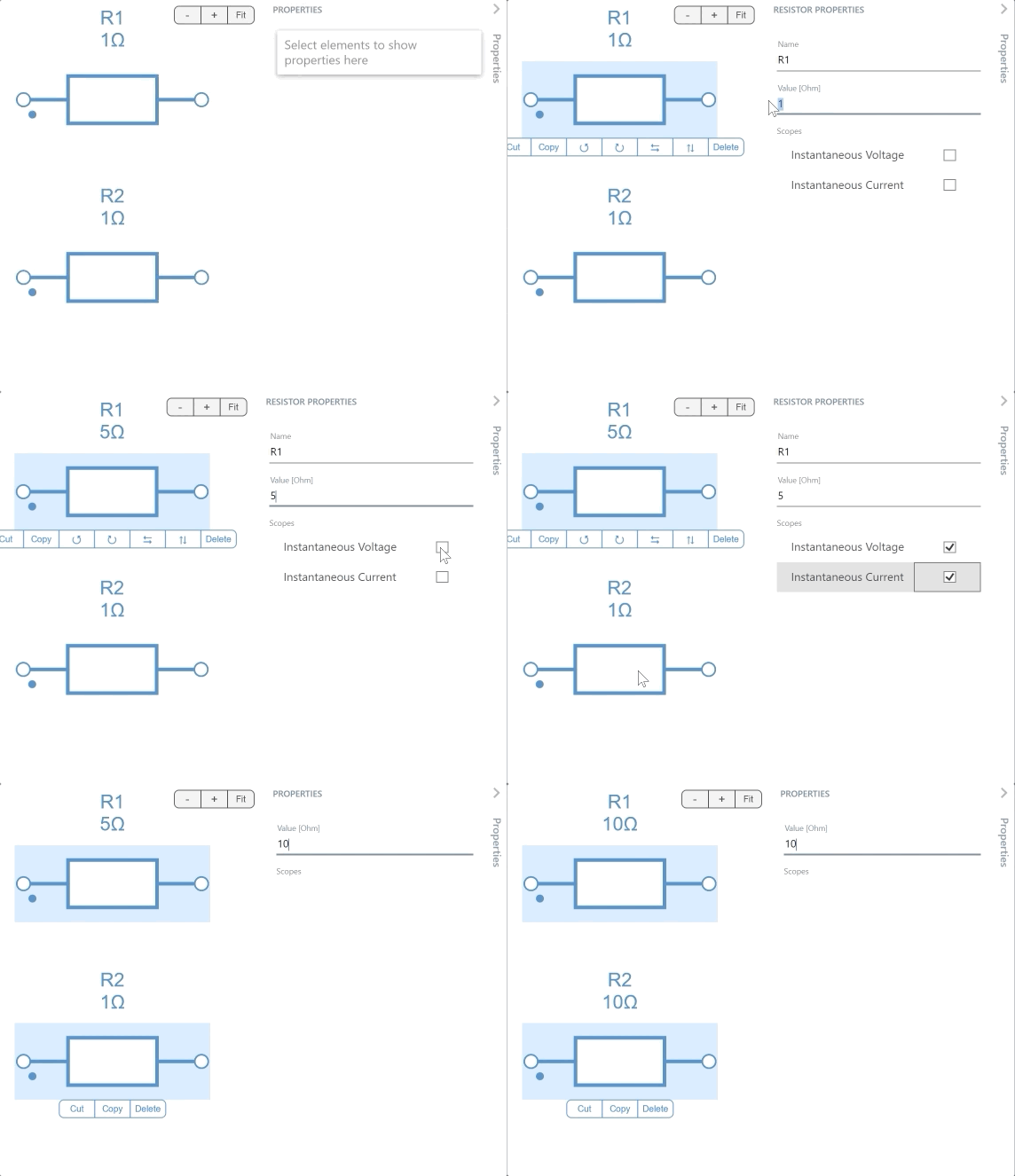
The Properties panel on the right-hand side lists the parameters and scopes of selected models. It is possible to select multiple models to change their parameters at once.

Model parameters syntax

Model parameters can now use metric units and mathematical expressions.

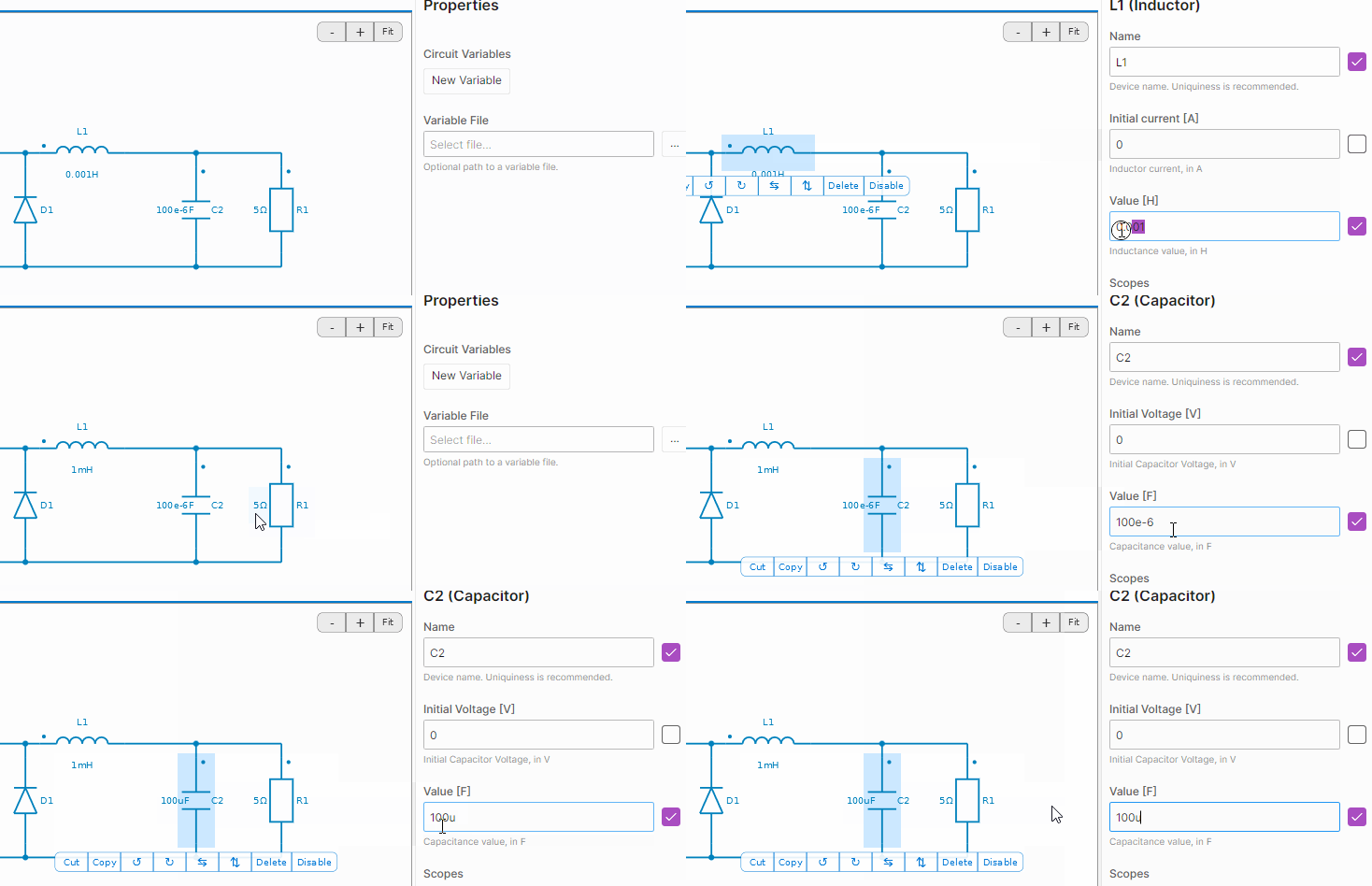
Accepted suffixes are:

Suffix	Coefficient
p	10E-12
n	10E-9
u or µ	10E-6
m	10E-3
k	10E3
M	10E6
G	10E9

Simple Mathematical expressions can also be used in parameter evaluations.

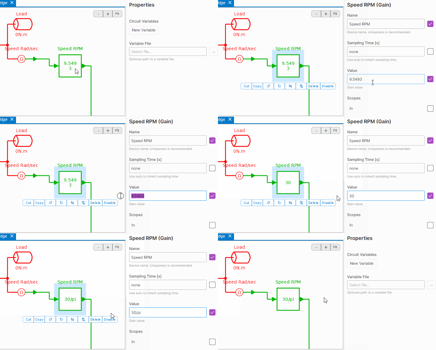
Basic operators (+, -, *, ^, !), constants (pi, e...) and math functions (sin,cos...) are supported.

Important

Expression are evaluated when simulation starts and a Syntax error is thrown if it can't be processed.

Variables

It is possible to define variables that can be reused in device parameter expressions.

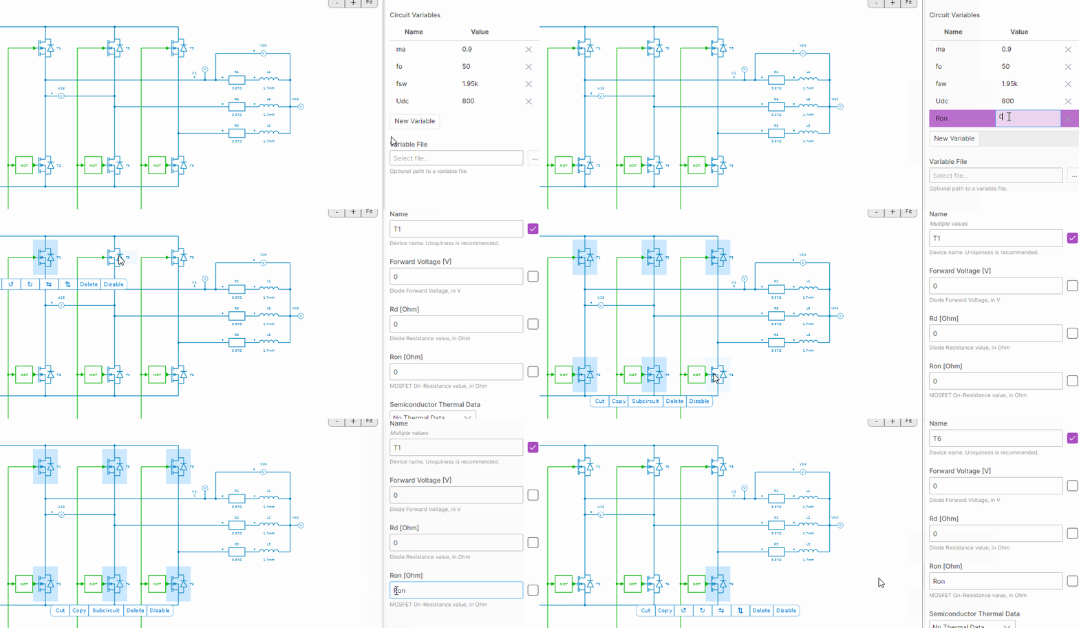
Variable File

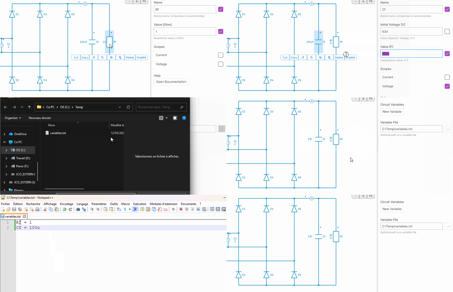
At the top circuit level, it is also possible to define additional circuit variables through a variable file.

The syntax is pretty simple:

• Comments are defined with //
• Variables are defined with the syntax : variable_name = variable_expression
• Expressions supports S.I. units (p,n,u,m,k,M) and mathematical expressions and functions (Ex: M = A * cos (X))

Result Tab

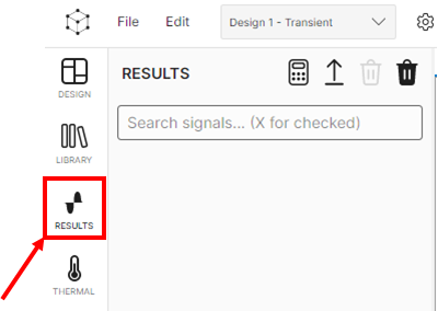
To access, the results of a simulation, select the results tab on the left side.

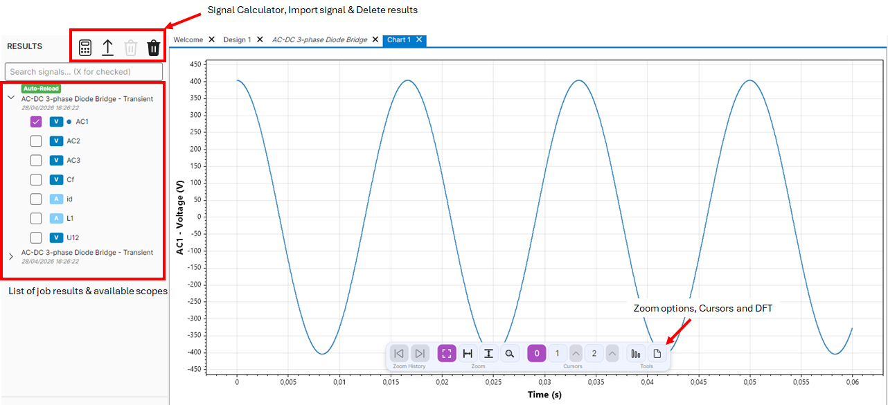
The result tab allows the user to handle simulation results with different features:

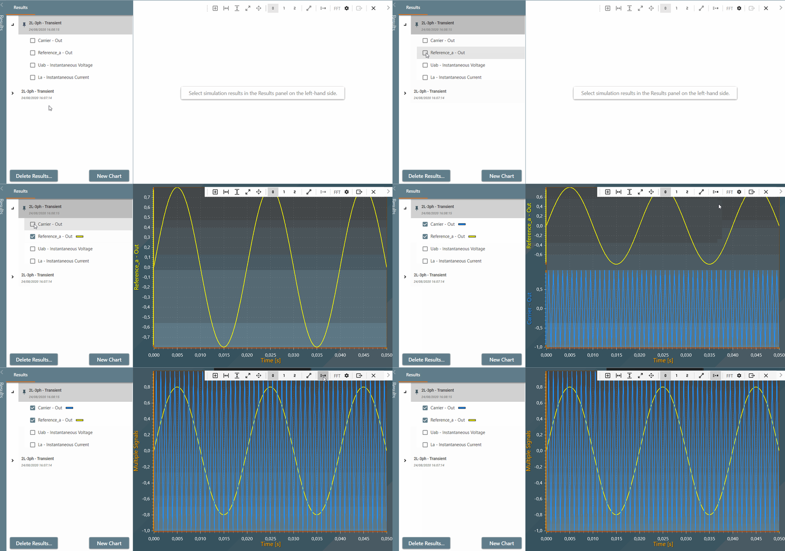
• select simulation results to display different charts through the result list located on the left-hand side of the tab;
• manage different zoom options, display time cursors, perform a Discrete Fourier Transform (DFT) and export the chart (png or csv) with the toolbar located on the bottom of the chart,
• open the signal calculator and apply one of the several available functions to the results,
• import results from CSV files, more informations are available in the Import an external .csv file section.

Select simulation results

Simulation results are listed on the left-hand side of the simulation result tab. The "top-one" with the pin symbol always points to the last simulation and the result display will automatically refresh after a new simulation is run.

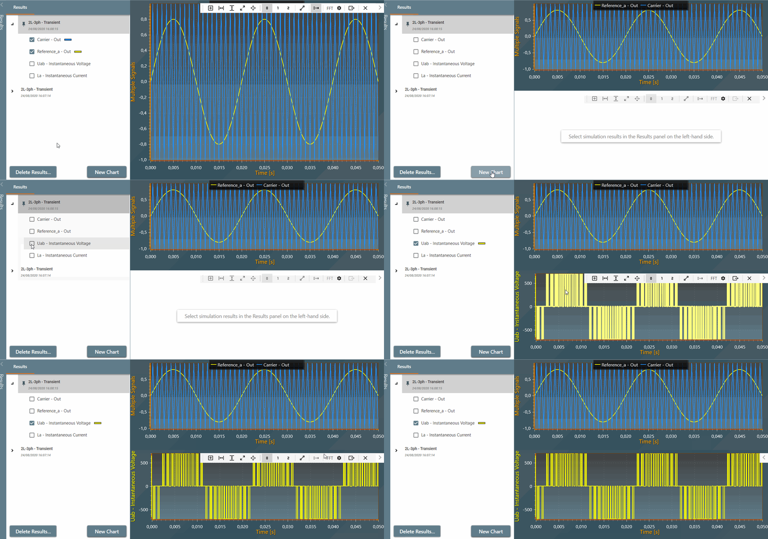
Charts pannel

Use the button New Chart to add a new empty chart in a new window.

Select a specific chart in the charts pannel to add new plots to this chart.

Select a specific plot in the charts pannel to access different options:

• Axis configuration and legend position,
• X and Y-axis min & max values,
• Add the job description to the signal label.

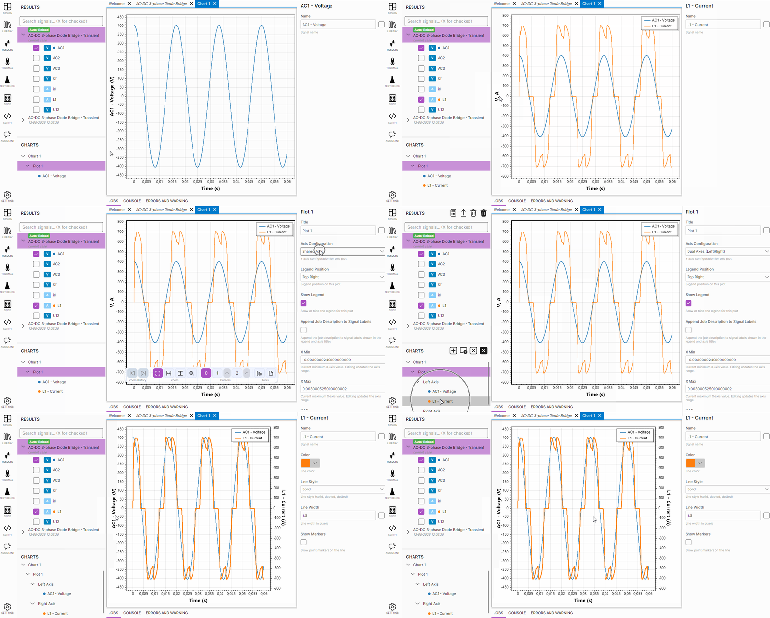Create a dual axis plot

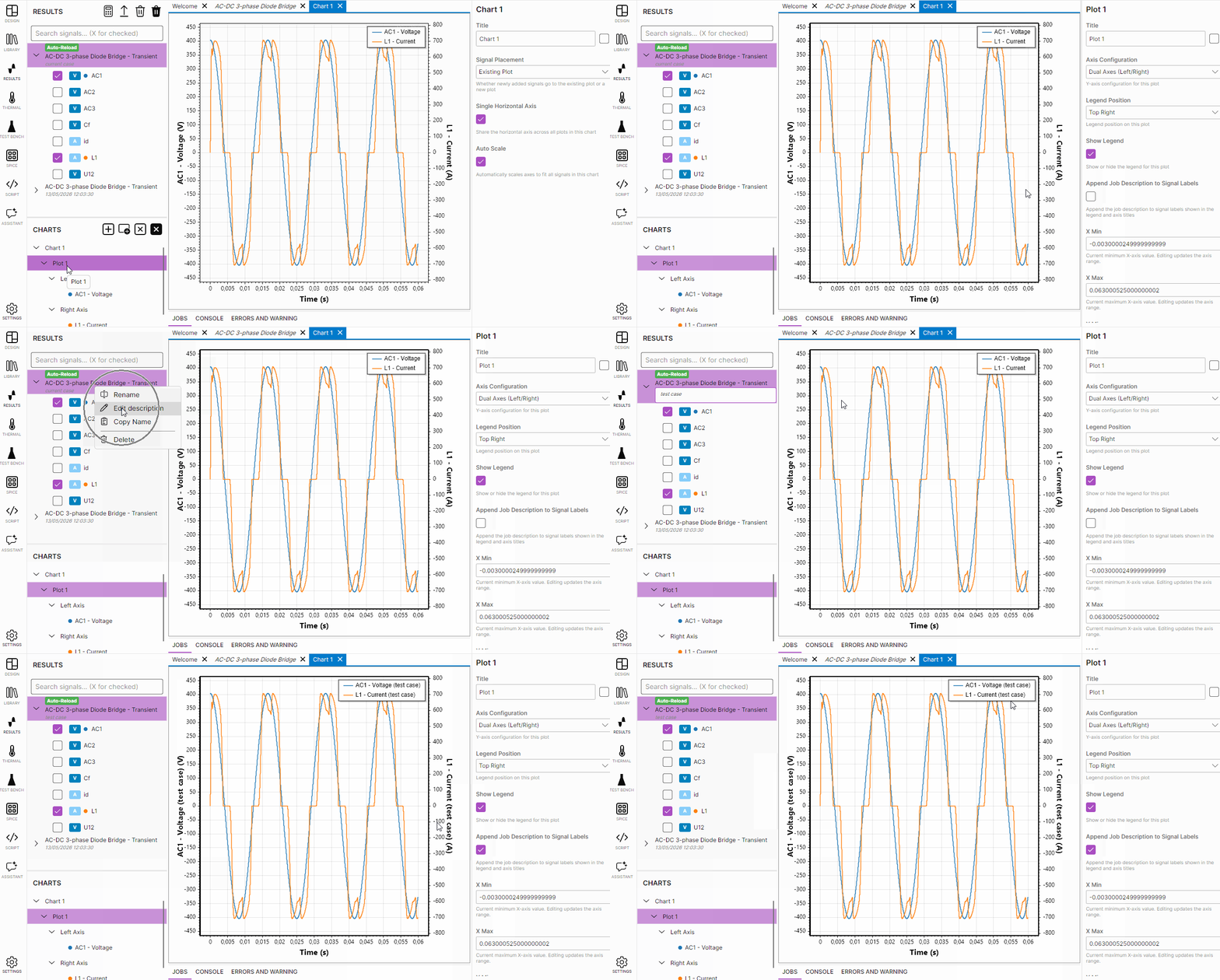Add a description

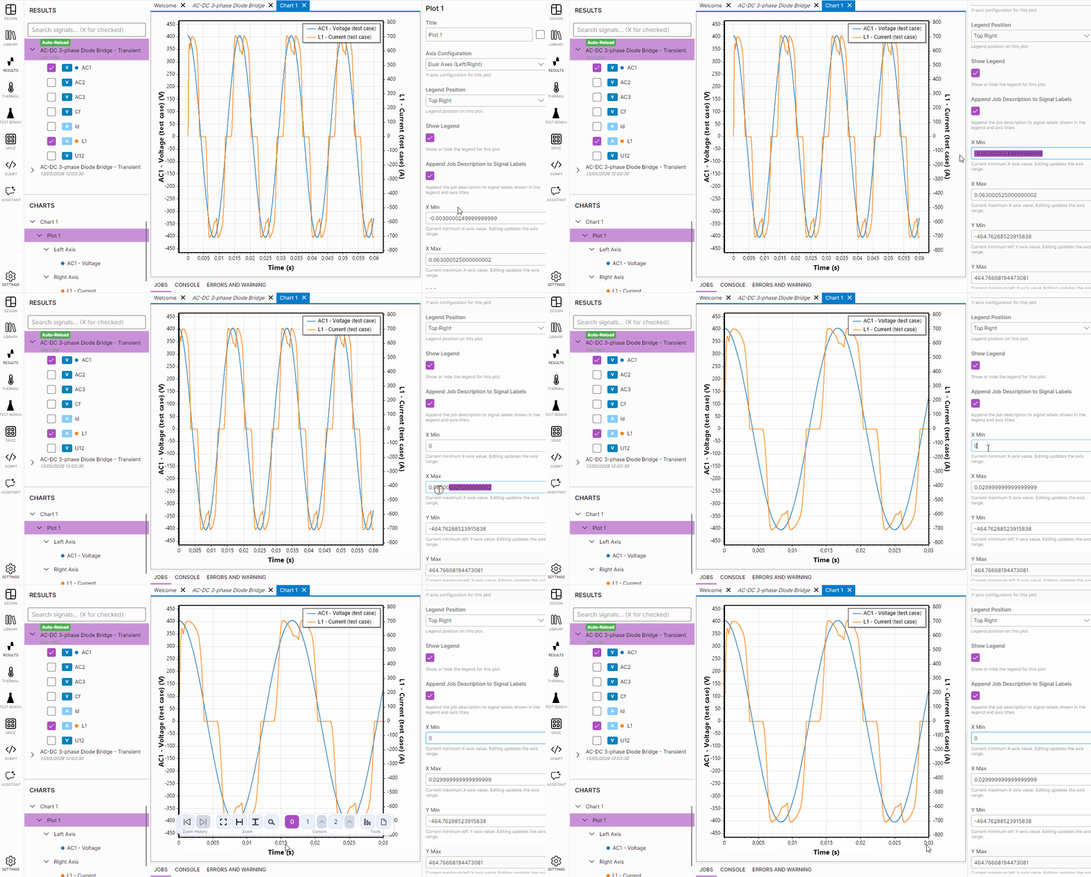Update X/Y axis min/max values

Select a specific scope in the charts pannel to access lines/markers style and colors.

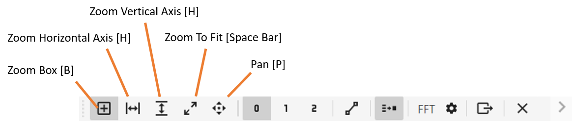
Zoom options

Different zoom options are available (shorcut in brackets):

Display cursors

One or two cursors can be activated providing x and y values and other information such as:

• the minimum, maximum, peak-to-peak (P2P) values between the two cursors,
• the mean and RMS values over the time period between the two cursors.

Important

It is possible to manually set the cursor position directly in the cursor measurement panel.

Note

By selecting the 'locker' button, the distance between the two cursors is maintained while moving a cursor.

Signal calculator tool

The Signal Calculator tool enables users to define, manipulate, and evaluate signal equations using existing signals from different jobs. This tool simplifies the creation of mathematical expressions by integrating signals and predefined functions.

How to use it?

1. Add signal variables

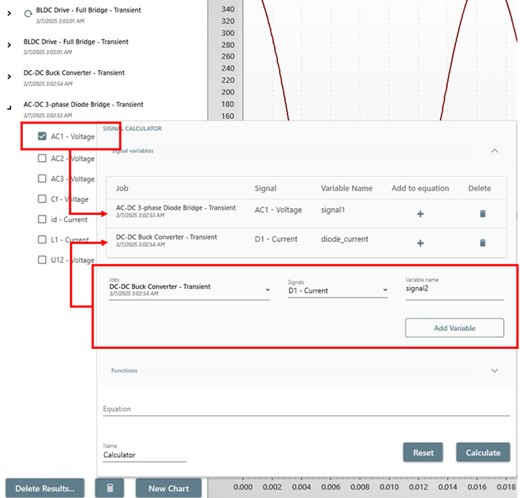
A signal variable is requested to use a signal in the equation. Users can add signal variables based on existing jobs and signals. Signal variables appear in a table where they can be renamed, added to the equation, or deleted. Users can also create signal variables using the button "Add".

• Select a job from the dropdown list.
• Choose a signal associated with the job.
• Enter a variable name to identify the signal in the equation.
• Select "Add" to include it in the list.

Note

The tool can automatically creates variables from displayed signals (checked signals) and add them to the table when selecting "Use Checked".

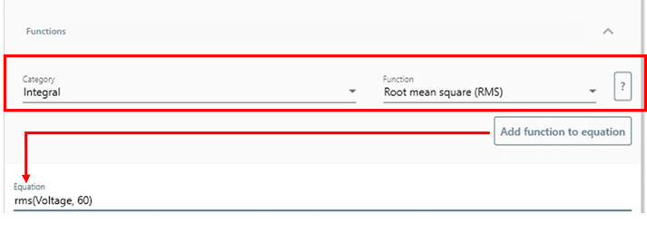
2. Adding functions

The tool provides a selection of functions categorized by type (Math, Trigonometry, Integral, Time-domain).

• Select a category from the dropdown list.
• Choose a function from the available options.
• Add the function to the equation by clicking "Insert function".
• A brief description is available for each function. For most functions, arguments can be signal variables, constants, or full expressions (with several signals). See the detailed description of each function.

Classic mathematical or logic operators are also usable:

Operator	Description
+	addition
-	subtraction
*	multiplication
/	division
^	raisextothepowerofy
<=	lessorequal
>=	greaterorequal
!=	notequal
==	equal
>	greaterthan
<	lessthan
&&	logicaland

Note

Signal Calculator functions supports composed functions: int(signal1 + signal2), ddt(signal1 + 2*signal2), int(ddt(signal1 + signal2)), moving_average(signal1 + signal2, 500) are usable formats.

The only exceptions are time-domain functions: delay(...) and t_window(...) must be used as the full root expression, and their first argument must be a simple signal variable (not a composed expression). Example allowed: delay(AC1, 1e-3) Examples not allowed: delay(AC1 + AC2, 1e-3), delay(AC1, 1e-3) + AC2, t_window(AC1 + AC2, 1e-3, 2e-3)

3. Build an equation

The equation is a mathematical expression built using signal variables and functions to calculate the new signal.

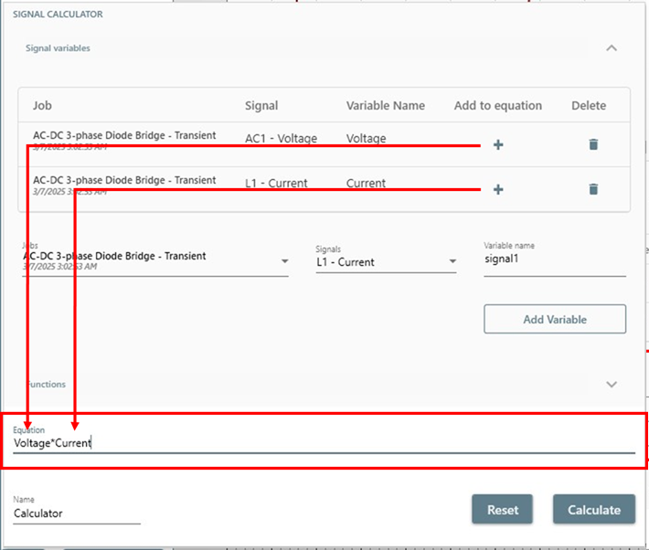
4. Calculate the signal

Once the equation is defined:

• Give a name to the calculation ("Calculator" by default).
• Select "Calculate" to execute the computation and generate the corresponding signal.

Note

If the process if completed, the new calculated signal will be automatically dispayed for visualization.

Note

If the is an issue in the definition of the signal (for example, at least one signal variable is necessary), an error message will be displayed in red.

Perform a Discrete Fourier Transform (DFT)

The DFT calculation performed in SIMBA computes each requested frequency (fundamental and harmonics) directly on the selected time window using a non-uniformly sampled DFT formulation (complex integral over the signal).

Two modes are available to perform this Discrete Fourier Transform:

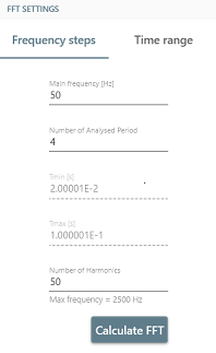
• Frequency steps: the user defines the first frequency (the fundamental), the number of harmonics to calculate and the number of periods to consider,
• Time range: the user defines the minimal and maximal time of the window to consider and the number of harmonics to calculate.

Frequency Steps mode

In the Frequency Steps mode, the DFT settings are defined with the following parameters:

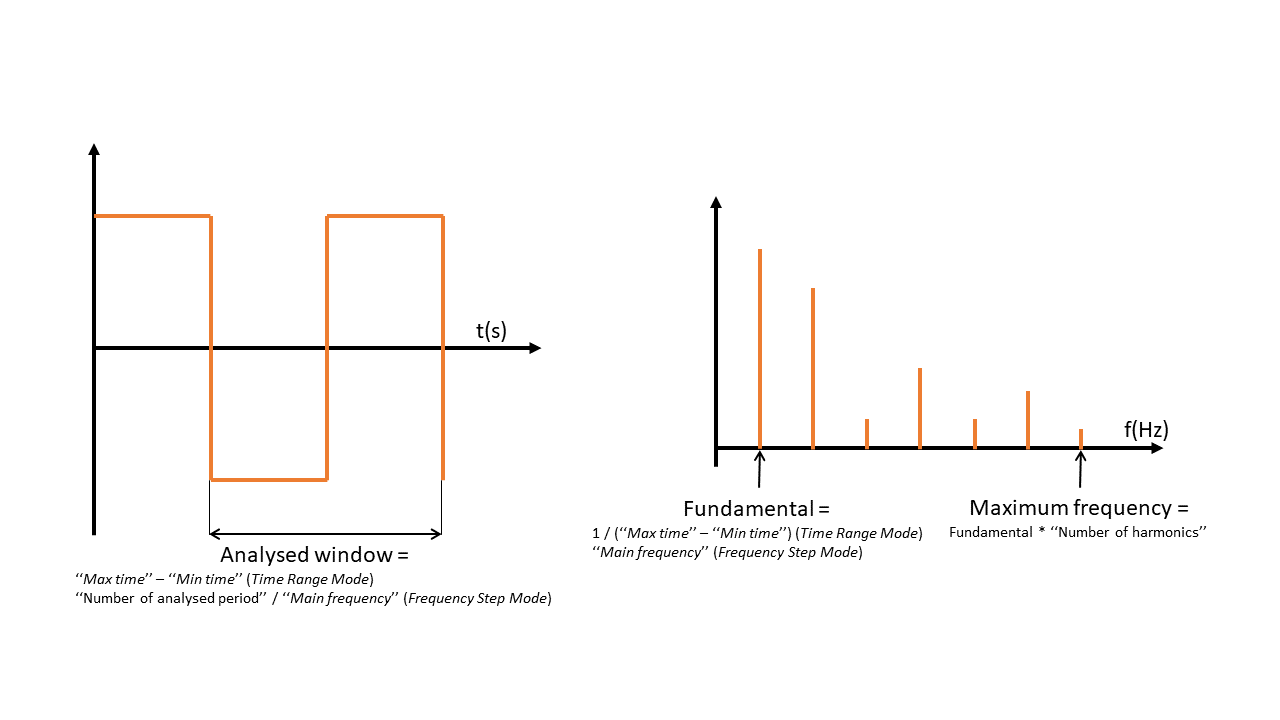
• Main frequency (in Hz): the frequency of the fundamental for the DFT calculation,
• Number of analysed period: defines the number of periods to scan,
• Number of harmonics: defines all the calculated frequencies (fmax = Main frequency * Number of harmonics)

Minimal and maximal time (in s)of the considered window are calculated from the other settings:

• Max time is the last simulation point,
• Min time is defined to have a width of Number of analysed period / Main frequency.

Time Range mode

In the Time Range mode, the DFT settings are defined with the following parameters:

• Min time (in s): the left border of the analysed window.
• Max time (in s): the right border of the analysed window.
• Number of harmonics: defines all the calculated frequencies (fmax = Number of harmonics / (Max time - Min time)).

In this mode, the Number of analysed period is 1 and the Main frequency is defined as 1 / (Max time - Min time)

Note

If the cursor mode is activated, Min time and Max time are derived from the position of the cursors: One cursor: Min time is the cursor position and Max time is the last simulation point, Two cursors: Min time is the postion of the left cursor and Max time is the position of the right cursor.

Algorithm considerations

The DFT is computed directly from the signal samples in the selected time window (no per-frequency resampling step is applied before the transform).

For sampled signals, SIMBA reconstructs the time axis from sampling information. For non-sampled signals, SIMBA uses the original time points.

The implemented formula is:

$$X(f) = \frac{2}{T} * \sum_s \int_t y(t) * \mathrm{e}^{-2j\pi*f*t} \cdot dt$$

where y(t) is the piecewise-linear interpolation of the samples on each segment s of the signal between [tmin, tmax].

For the DC component, we use the mean definition.

Import an external .csv file

The result view allows to import .csv result files from other software into SIMBA.

SIMBA supports two different .csv formats:

• "Single Time Column Format": the first column of the .csv file is the time, the others are the different measurements,
• "Multiple Time Column Format": each odd column is the time, each pair column is a specific measurement.

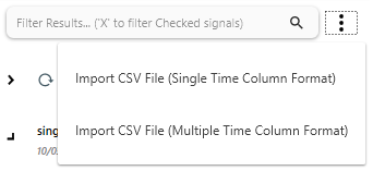
To add a new chart using an external .csv file, click on the button - - next to the filter view, choose the desired csv format and select the file to load. It will create a new chart with all the signals from the .csv file.

Note

Authorized format for the .csv files:

• "Single Time Column": Time,Out1,Out2 / Example here
• "Multiple Time Column": ime,Out1,Time,Out2 / Example here

Test Bench Tab

Test benches include various parametric analysis and model characterization tools. Test benches are designed to automate the modeling and simulation of power converters. Single parameter sweep are currently available. More test benches will be added soon.

Views option

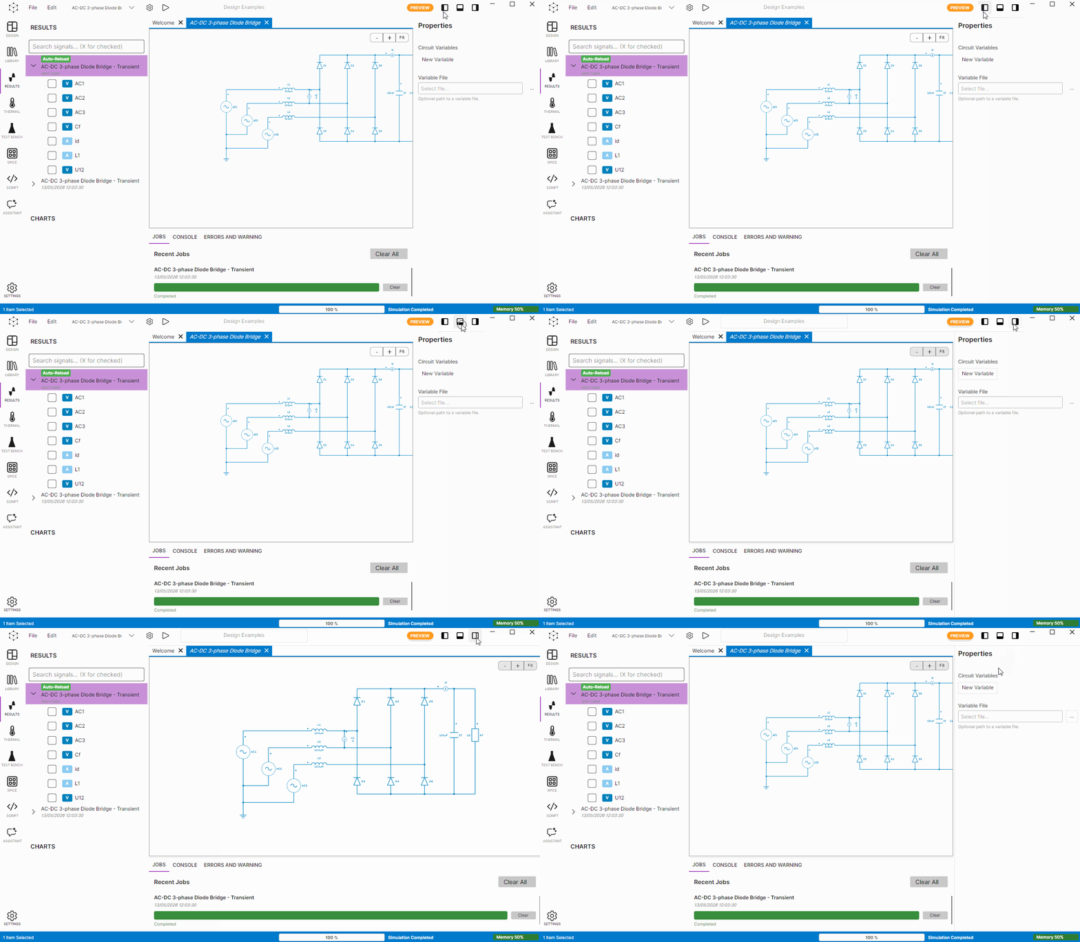
The Top-Right corner proposes 3 options to show / hide the different pannels (design/console/properties). Also, it is possible to extend/reduce their size using drag & slide with the border.

Subcircuit and User-Defined Libraries

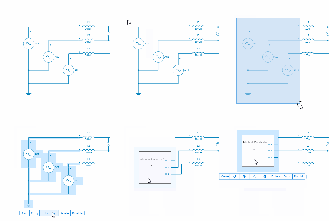
Circuit can be simplified by grouping models into subcircuits. Subcircuits are stored in User-Defined Libraries bound to a project.

To create a new library, select the devices to encapsulate in the subcircuit. Then, use the button in tool-tip bar to create a new subcircuit.

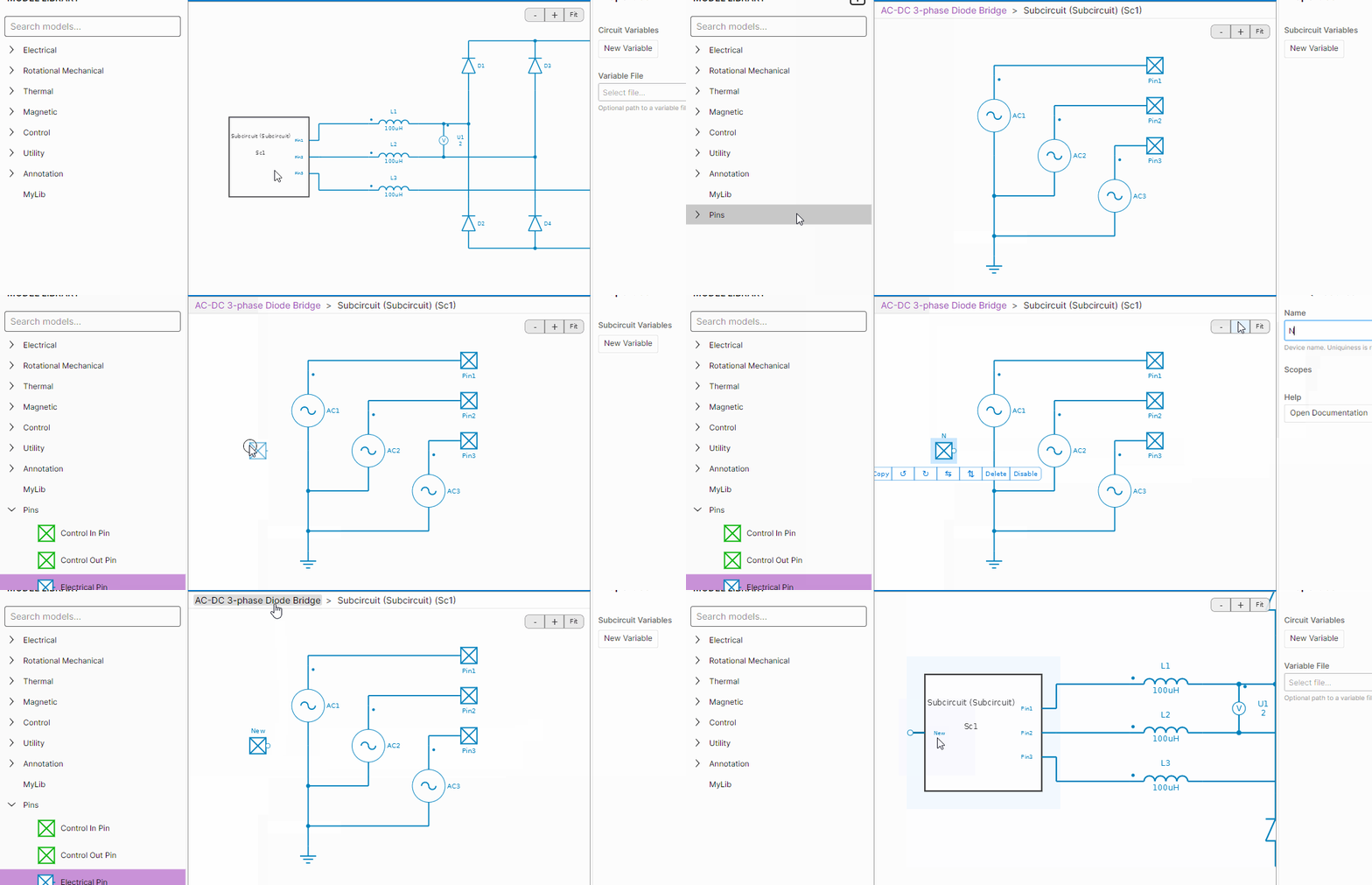
To edit a subcircuit, simply use the Open button. When editing a subcircuit, the Pins library is available. Pins are typed (Electrical, Control, and Mechanical) and are used to interface subcircuits.

When selecting a subcircuit device in a design, the Properties panel includes Number Of Subcircuits In Parallel. Set this to the number of identical subcircuit instances to simulate in parallel. Each instance shares the same definition and parameters, and corresponding pins across instances are tied together. Instances are numbered with a suffix (_1.._N) in results and scopes. The value is clamped between 1 and 20.

Edit the subcircuit

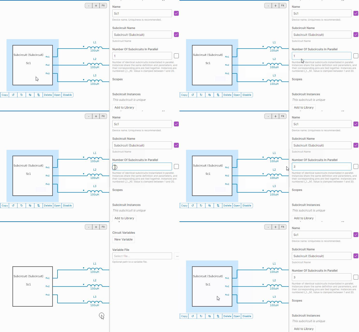Change the number of parallele subcircuits